Parallel Programming with Scilab

A Brief Tutorial

Konstantin Tretyakov

October 5, 2006

When you are doing data analysis you might quite often find yourself in a situation where you need to run some simple but moderately time-consuming procedure many times with different parameter values. Finding the best regularization coefficient for a statistical model, calculating all pairwise edit distances between sequences, plotting ROC curves, doing randomization tests, monte-carlo integration, preparing a video, ... — in all of these cases you deal with essentially the following code

for x in range(...):
	result[x] = F(x)

where F is some procedure whose running time is not completely ignorable. Usually the whole loop will take from a pair of hours to maybe a day to run, and it is, so to say, "tolerable". You can leave the calculation running for the night and get your results the next day.

However, once you end up recalculating something for the fifth night, you get the idea, that if you could only make the thing ten or twenty times faster, you would reduce the running time to some 20 minutes, and that would allow you to "play" with your code in a much more comfortable, nearly interactive manner.

There are several approaches you could employ: optimizing the code, rewriting it in C, applying sophisticated algorithms, using the grid, etc. All of them have their costs and benefits. Here I shall show you a simple way to parallelize your program using the Parallel Virtual Machine package, and run it on a cluster of computers (in particular the Linux computer class of Liivi 2, or the computers in the room 314). The major benefit of this approach is that it's relatively simple to use in a wide variety of settings — it might be considerably easier to parallelize your loop with PVM than to rewrite the algorithm or to convert it into a batch of grid jobs. Besides, you can use PVM together with any of the above optimizations.

To make things specific I'll present a "tutorial-like" step-by-step illustration. We'll be dealing with the problem of estimation of the effect of regularization on linear regression with Scilab. The choice of the example problem was somewhat random, but I hope it's reasonably simple and the result is enlightening. Scilab (or Matlab) is often the language of choice for such problems and the fact that you can use PVM with Scilab impressed me strongly enough to be willing to share this impression. Note, however, that PVM can be used with pretty much any language out there.

... and yes, those not interested in the example may just skip the following section and go directly to the PVM part.

Example Problem

Suppose you are willing to estimate a linear regression model

y = b₁x₁ + b₂x₂ + ... + b_mx_m = b^Tx

on a set of datapoints {(x_i1, x_i2, ..., x_im; y_i)}. That is, you've got several vectors x and the corresponding values of y and you are interested in finding the coefficient vector b describing the linear relation between x and y.

It is well known, that the least-squares (maximum likelihood) solution for b is

b = (X^TX)^-1X^Ty

where X is the matrix with rows containing training vectors x_i and y is a vector of corresponding values for y_i.

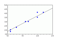
For example, the following Scilab code finds the best b for a one-dimensional dataset and plots the result:

X = [1.1; 1.1; 1.3; 1.6; 1.7; 2.0; 2.0; 2.2];
y = [2.0; 1.8; 2.3; 3.0; 3.0; 3.5; 4.1; 4.1];

// Solve for b
b = inv(X'*X)*X'*y;

// Plot points
plot(X, y, '.');

// Plot regression line
t = 1:0.1:2.5;
plot(t, b*t, 'k');

It is known that the coefficients b of a linear regression model may be unstable, especially if the amount of data is small or the noise is large. That is, the resulting b may depend on the noise too heavily to be useful. A common trick, called regularization is supposed to address this issue: we solve for b as

b = (X^TX + λI)^-1X^Ty

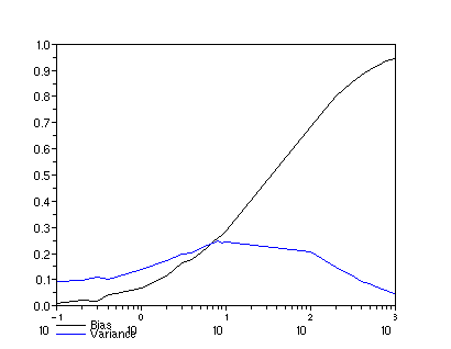
where I is the identity matrix and λ is a small regularization parameter. The regularization parameter should make b more stable and less dependent on the noise, with a price of a slightly increased bias (i.e. b does not give the "exact" solution to the regression problem any more).

This all is theory, and it might be interesting to know exactly how λ affects the bias and the variance of the coefficients b, for some specific nonzero value of b. We can write a simple program that does it. For each value of λ we'll generate several random datasets, solve the regression problem, and take note of the standard error and standard deviation of the obtained solution. The outer loop of the program might then look approximately like that:

example.sce
getf("estimate.sci");

// Evaluate bias and variance for these lambdas
lambdas=[0:0.1:0.5 1:10 100:100:1000];

b_bias = []; b_variance = []; // Store results here

for lambda=lambdas // For each lambda
  [b_bias($+1) b_variance($+1)] = estimate(lambda);
end

and the code of the estimate function in the inner loop is available in the file estimate.sci. If you want to test it, download the files example.sce and estimate.sci to your home directory and invoke scilab there:

> $SCI/bin/scilab -nw -f example.sce

This is a reasonably simple example and it's running time is about a minute. But be it something more interesting than plain linear regression, it might easily run in over several hours. In this case you'd gain quite a bit from parallelization.

PVM

Parallel Virtual Machine is a software package that allows to use several machines as a single "virtual machine" with several processors, where you can spawn processes and let them communicate with each other. It comes already installed with scilab so I'll omit the installation details. You will need to perform some setup though.

Setup

In order to use PVM you need to select a cluster of computers preferably sharing a filesystem. Here we'll use the machines in room 314 (kirss, murel, tikker, vaarikas, pihlakas, aroonia, toomingas), emu and kotkas. All of them mount your shared home directory as well as the /group directory. Scilab is installed in /group/software/general/scilab-4.0, and PVM — in /group/software/general/scilab-4.0/pvm3. There are four things you need to do:

Setup the SCI, PVM_ROOT and PVM_ARCH environment variables in your login script.
For example, if you use bash, add the following lines to your ~/.bashrc:
```
export SCI=/group/software/general/scilab-4.0
export PVM_ROOT=$SCI/pvm3
export PVM_ARCH=LINUX
```
Setup password-less login between the hosts.
```
> cd ~/.ssh
> ssh-keygen -t rsa
     -- Save the file as id_rsa, use empty password
> cat id_rsa.pub >> authorized_keys
```
Test it by ssh-ing onto other hosts. You should not be asked for a password. For more information read man ssh.
Prepare a PVM hostfile. A hostfile specifies the hosts which will constitute the virtual machine, as well as some options. If you're interested in details, you may read this, however, for our case you should just use the file /group/software/general/scilab-4.0/pvm3/doc/hostfile. Copy this file to ~/.pvmd.conf
Now run PVM.
```
> $PVM_ROOT/lib/pvm -nkirss.at.mt.ut.ee ~/.pvmd.conf
```
Where you should use your host name instead of kirss.at.mt.ut.ee.^[1] If everything goes fine you should see a pvm> prompt. Enter the conf command and you should see a list of hosts. You can use the halt command to stop PVM (using quit or Ctrl+C will just close the console, but leave the PVM daemon running).

PVM Programming

Now you can do some PVM programming. Of the whole set of PVM functions you need only 4-5 to get started. Here are some examples:

The shortest PVM program

myid = pvm_mytid(); // Find out your id, involve in a PVM session
pvm_exit()	;   // Leave PVM

Spawning a subprocess (suppose this is saved as ~/test.sce)

p = pvm_parent();  // Who is my parent?
if p == -23 then   // No parent? Then I'm the parent.
    // Spawn one copy of this script
    // Only specify scripts by full path! Also don't forget the "nw"!
    pvm_spawn("/home/me/test.sce", 1, "nw"); 
end
pvm_exit();        // Leave PVM
quit();            // Otherwise the spawned process won't terminate

Communicating (suppose this is saved as ~/test.sce)

p = pvm_parent();
if p == -23 then
    pvm_spawn("/home/me/test.sce", 1, "nw");
    data = pvm_recv(-1, -1);  // Receive data from the child
    printf(data);
else
    pvm_send(p, "data", 1);   // Send data to parent
end
pvm_exit();
quit();

Parallel FOR-cycle

The examples above should already give an idea of how to paralellize the for-cycle of the example problem. The master process will spawn a separate subprocess for each λ and collect the results:

example_pvm.sceBASEDIR="/home/me/pvm/";
getf(BASEDIR + "estimate.sci");

lambdas=[0:0.1:0.5 1:10 100:100:1000];
n = length(lambdas);

// ------------ Code for the master process ------------
function [b_bias, b_variance] = master()
    // Spawn child processes
    [tids, nt] = pvm_spawn(BASEDIR + "example_pvm.sce", n, "nw");
    
    if n <> nt then
        printf("Error\n"); return; // Failed
    end

    // Distribute tasks
    for i=1:n
        pvm_send(tids(i), [i, lambdas(i)], 1);
    end

    // Collect results
    for i=1:n
        b = pvm_recv(-1, -1);
        b_bias(b(1)) = b(2);
        b_variance(b(1)) = b(3);
    end
endfunction

// ------------ Code for the slave process ------------
function slave()
   // Receive task
   task = pvm_recv(pvm_parent(), -1);
   
   // Calculate
   [b, v] = estimate(task(2));

   // Send result
   pvm_send(pvm_parent(), [task(1), b, v], 1);
endfunction

// ------------ Main ------------
if pvm_parent() == -23 then
    [b_bias, b_variance] = master();
else
    slave();
end
pvm_exit();
quit();

To test it, download the file to the same directory where you saved estimate.sci, correct the path in its first line, and execute

> $SCI/bin/scilab -nw -f example_pvm.sce

In my case the speedup was approximately 7-fold, which is quite nice for many cases. With a little thought you can optimize the thing even more. You can also run the script on the cluster of computers in the linux class of Liivi 2^[2], which contains more machines. And in the extreme case you might ask for a large cluster on the grid.

PVM vs MPI

The discussion would not be complete without noting that there is a widely popular alternative to PVM, called MPI, which could be used to parallelize programs in a similar manner. In most cases the choice of technology is a matter of taste, so when I say that I find PVM easier to use for simple cases, it only reflects a rather subjective opinion of mine. When you use Scilab, however, PVM is your only easy choice, and fortunately it does the job really nicely.

Conclusions

The main idea of the exposition above was to show that parallelizing a Scilab program can be enormously simple, so simple that it's often worth a try even if you would otherwise be ready to wait some hours for your script to complete. Hopefully the reader has got the point so there's not much to write for the conclusion. And as for the result of the example problem, here's how the bias and variance depend on the lambda, think about it:

Footnotes

The reason for that, as well as the reason for having the IP addresses in the hostfile is that the machines in room 314 are configured to map their hostnames to 127.0.0.1 instead of their true IP, which confuses PVM.
Scilab is installed there at /usr/lib/scilab-4.0. The appropriate hostfile is this.